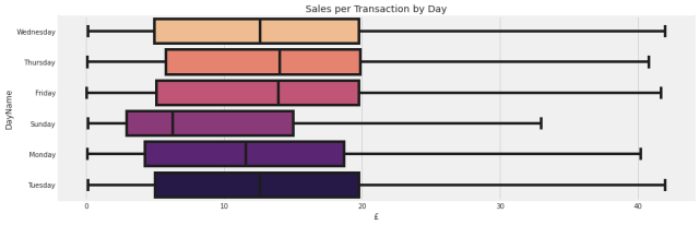
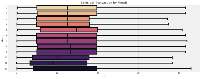
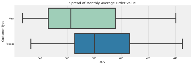
Today, we’ll work with the retail transactions data we cleaned and processed in a previous post. After detecting and treating outliers using Tukey’s method and winsorization, we’ll uncover purchase patterns across different time slices and define Pareto – or the 20% of products and customers driving 80% of sales. We’ll compare new and returning customers, which we’ll define as first-time purchasers and customers purchasing again within a month, respectively. Classifying new and returning customers helps us understand how customer acquisition and retention rates change over time and how purchase habits, like average order value (AOV), compares between the two groups.
We’ll then create a dataframe of juicy metrics, including recency, frequency, monetary value (RFM), average and total quantity, AOV, and 90th and 50th percentile of days-between-purchase by customer. While we we’ll use only a few of them for the purpose of classifying churn risk, let’s save and keep them handy for future modeling. If you’re interested in learning more on RFM, check out our previous post on RFM metrics and segmentation / clustering.
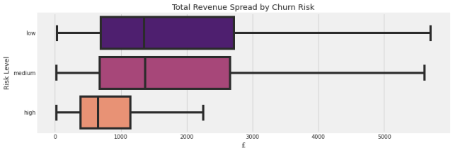
Lastly, we’ll define churn risk by customer. Since we’re working with retail e-commerce data, the type of churn is voluntary, continuous, and non-contractual. We’ll define a function to identify high, medium, and low churn risk by customer. We’ll also visualize purchase differences by churn risk. Based on customers classified as high risk of churn, we’ll see that £828337.83 in revenue is at high risk of being lost. Classifying churn risk allows us to allocate resources where they’re needed most. For example, we can intensify sales, marketing, and product activities aimed at high risk churn customers in order to retain them.
Code below and in more readable form on colab and GitHub.