Guns: Time Series Analysis and Forecast

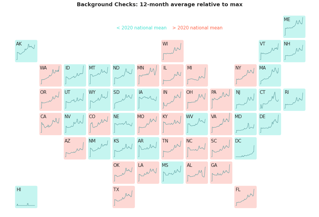
Today, we’ll do a deep-dive time series exploration and SARIMAX forecast using data on gun backround checks in the U.S. It was inspired by a recent Berlin Time Series Analysis meetup I attended and previous analyses done by the New York Times and BuzzFeed. The purpose is to:

• Understand, predict, and forecast gun sales in the U.S.
• Explore and visualize time series data from multiple perspectives

Background check data originates from the FBI’s National Instant Criminal Background Check System (NICS). Original data is available as a pdf. If you’d like to extract the csv from the pdf directly, you can do so using BuzzFeed’s parsing scripts or Tabula. According to the data pdf, “These statistics represent the number of firearm background checks initiated through the NICS. They do not represent the number of firearms sold. Based on varying state laws and purchase scenarios, a one-to-one correlation cannot be made between a firearm background check and a firearm sale.” Important things to keep in mind for our analysis:

• We focus on background checks by month, state, and gun type, namely long guns, which include rifles and shot guns, and handguns.
• We exclude permit check/recheck as regulations vary widely by state
• Also excluded are ‘other’ gun background checks
• The FBI’s NICS figures only include commercial gun sales and exclude private gun sale, which often don’t undergo a background check and represent a sizeable portion of total gun sales. Additionally, many background checks are carried out for concealed carry permits, not gun sales (e.g., Kentucky runs a new check on each concealed carry licence holder each month).

To convert background checks to sales (number of units), we apply the multiple gun sales factor (MGSF) multiplier found in Jurgen Brauer’s Small Arms Survey, which is based on interviews with gun shop owners: multiply background checks for handguns by 1.1, long guns by 1.1, and multiple guns by 2 (page 44). Because state laws and individaul transactions differ, sales between states cannot be directly compared. Despite those caveats, the FBI’s NICS numbers are widely accepted as the best proxy for total gun sales in a given time period. Additionally, to adjust sales for population growth, we’ll pull monthly U.S. population data from Federal Reserve Economic Data (FRED).

The heart of this analysis is exploration and visualizations of gun sales per 100,000. While it’s not always necessary to apply all of these visualization for every time series you encounter, we highlight them here to showcase multiple aspects of time series data. Finally, using the Box-Jenkins framework, we’ll walk through identification, estimation (SARIMAX), and model diagnostics, including fitting a prediction and forecast. Future areas for improvement:

• Long-gun vs. handgun: we only dig into total sales of all types of guns, it would be interesting to understand state-level and national trends between long guns, which are traditionally bought for hunting, and handguns, which are used more for self-defense
• Context: get more context from policy experts to understand what constitutes a reasonable forecast error in this specific case. MAPE has its own disadvantages so consider other metrics that social policy experts use
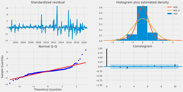
• Distribution of Residuals: with the Jarque-Bera(JB) test and its low (<0.05) p-value Prob(JB), residuals are not entirely normally distributed. We could also see this in the QQ plot. We could check if removing more outliers improves this.
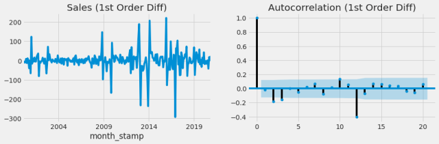
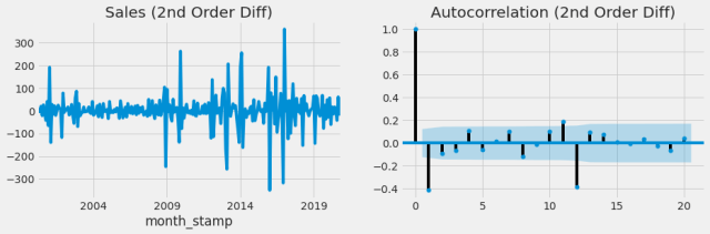
• Stationarity: Our differenced data is only weakly stationary. We can see this in the higher variance in the earlier part of the series. Apply and compare other log transform, n-level differencing, seasonal differencing, or square root adjustments.
• Incorporate exogenous variables: Incorporate exogenous variables (e.g., unemployment, poverty, crime rates, legistlation, covid, etc)) into SARIMAX.
• Social Policy: Translate the model selection/optimization rationale, evaluation metrics (e.g., MAPE), predictions and forecasts into specific social policy impact so that it’s helpful to understand for legilslators and the public.

We also include a list of resources at the end. You can find our code with explanatory notes and findings at our Git and below as a gist along with images.

Lets’ dig in and see what we find!

Table of Contents

1. Introduction
2. Install and Import Packages
3. Access NICS Background Checks Data
4. Missing Values
5. Exploratory Data Analysis
   5.1. Background Checks by State
   5.1.1. Boxpatch Map
   5.2. National Sales
   5.2.1. Observed
   5.2.2. Rolling Mean with Rolling Standard Deviation
   5.2.3. Rolling Median with Rolling Quantiles
   5.3. Population-Adjusted National Sales
   5.3.1 Rolling Mean with Rolling Standard Deviation
   5.3.2 Monthly Sales by Year
   5.3.3. Monthly Cyclic Sales by Year
   5.3.4. Monthly Sales Yearly Seasonality
   5.3.5. Distribution of Monthly Sales by Year
   5.3.6. Monthly Sales by Year Bar
   5.3.7. YoY Monthly Sales Growth
   5.3.8. YoY Monthly Sales Share Growth
   5.4. 2020 Outlier Adjustment
   5.4.1. Autocorrelation
   5.4.2. Autocorrelation Function (ACF)
   5.4.3. AD Fuller (ADF) Test
6. Identification
   6.1. Seasonality
   6.2. Stationarize
   6.3. Identify AR Order
   6.3.1 Partial ACF (PACF)
   6.3.2. AIC and BIC
   6.4. Identify MA Order
7. Estimation
   7.1. SARIMA
   7.2. SARIMAX
8. Model Diagnostics
   8.1. Plot Diagnostics
   8.2. SARIMAX Summary
   8.3. Prediction (In-Sample)
   8.3.1. Evaluation
   8.4. Forecast (Out-of-Sample)
9. Future Areas for Improvement
10. Resources