My wife caught the investing bug. She recently put together a portfolio of healthcare, consumer (cyclical and defensive), technology services, and media companies that she’d like to invest in long-term based on their business model / fundamentals, earnings and cash flow outlook, and current (under)valuation:
- Norton LifeLock (NLOK)
- Keysight (KEYS)
- BioNTech (BNTX)
- Quest Diagnostics (DGX)
- Disney (DIS)
- Kroger (KR)
- Pinduoduo (PDD)
- Peloton (PTON)
- NetEase (NTES)
- Bristol Myers Squibb (BMY)
In this post, I’ll walk through how I helped her optimize, that is, find the best weights (allocation) for her investment to maximize risk-adjusted returns based on her risk tolerance.
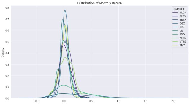
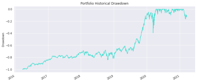
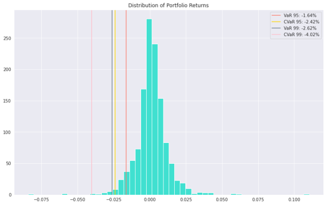
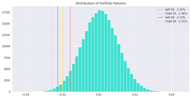
We’ll first collect price data going back 5 years using the yahoo finance API and take a look at company returns, correlations, and distributions. Before creating an optimal portfolio, we’ll construct an equal-weighted (naive) portfolio and understand expected portfolio returns, volatility, and tail risk, including value-at-risk (VaR) and conditional value-at-risk (CVaR) at 95% and 99% confidence.
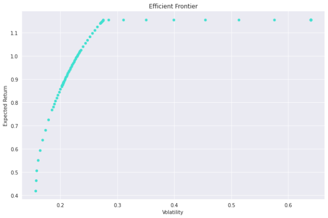
We’ll then dig further to uncover simple Markowitz-optimized portfolios. To get more optimal weightings, let’s first revisit our inputs – expected return and covariance. Since returns have fluctuated significantly, particularly over the past year of the pandemic, let’s exponentially weight returns to give more weight to more recent returns of the past 6 months. Additionally, the sample covariance we calculated for the equal-weighted portfolio isn’t very efficient because it overweights extreme events – even small differences in covariance can have a significant impact on optimal weights. Covariance shrinkage is often used in practice to address this. It combines the sample covariance matrix with a structured estimator, to reduce the effect of erroneous weights. To improve our optimization, let’s apply covariance shrinkage using the Ledoit Wolf method to get an efficient covariance.
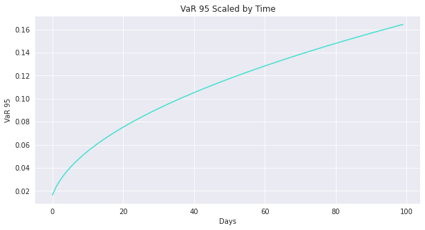
We’ll create maximum Sharpe Ratio (MSR) and global minimum variance (GMV) portfolios. Since MSR can be inconsistent – optimization is sensitive to expected return, which is difficult to estimate with high confidence – we’ll opt for the GMV portfolio. We’ll also see how cumulative returns from all of the portfolios we constructed compare to that of the S&P500. Finally, to better understand how our GMV portfolio could perform in the future, we’ll run a Monte Carlo simulation with 1,000 simulations to arrive at a parametric VaR and CVaR of simulated future returns. As we’ll see, one caveat of GMV is that it tends to overweight low-volatility components. To address this, we’ll make minor tweaks to the GMV weights to arrive at our final portfolio.
Future areas to explore:
- Apply robust optimization methods like Black-Litterman
- Incorporate more realistic, time-varying volatility estimates using GARCH models (similar to what we did in prior posts on Moderna, Spotify, and AbbVie here, here, and here).
Code below and in more readable form on colab and GitHub.